Editor’s note: This post is part of a series on “The Great Indian Poverty Debate 2.0”, discussing two new studies with conflicting estimates of the evolution of poverty in India. We’ve invited both sets of authors to offer their take. Sutirtha Sinha Roy and Roy van der Weide start off, to be followed by Surjit Bhalla, Karan Bhasin, and Arvind Virmani with their more optimistic view.
Official estimates of poverty in India are derived from the National Sample Survey (NSS) household consumption expenditure survey (CES). The most recent CES was compiled back in 2011, so to estimate how poverty in India has evolved since then alternative sources of data (and accompanying prediction methods) are required. Earlier this month two working papers came out, coincidentally within a day from each other, that produce estimates of poverty for India using different sources of data. For 2019, estimates of extreme poverty headcount is estimated to be over 10 percent in one study and 5 percent in the other. In this blog post, we reflect on the dramatically different poverty estimates produced by each paper, and the source of the discrepancy.
The first of these studies is a World Bank working paper by the authors of this blog (henceforward referred to as RR), which uses a new household consumption expenditure survey (the CPHS) collected by the private sector to measure consumption poverty. The CPHS is the first household survey collecting household expenditure data since the official CES round of 2011. Its expenditure questionnaire is, however, not readily comparable to that of the CES. For this reason, RR estimate the relationship between CPHS and CES household consumption and use this to convert CPHS consumption data into NSS-compatible consumption data – such that estimates of poverty and inequality obtained using the CPHS for the period 2015-2019 can be compared against historical poverty and inequality estimates until 2011.
The second study is an IMF working paper by Surjit Bhalla et al. (henceforward referred to as BBV), which uses state level GDP growth data to project mean household consumption growth under the assumption that state inequality levels have remained unchanged over this time time-period (as the state GDP data does not offer an any information on distributional changes). For a comparative summary of the two papers, we refer the interested reader to a recent blog post by Justin Sandefur (2022).
Figure 1: Replicating headcount estimates of Bhalla, et al (2020)
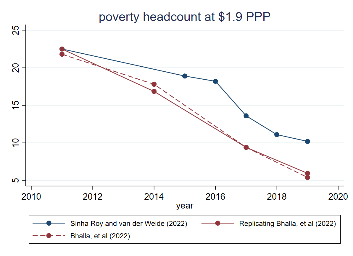
Notes: Our replication of Bhalla et al. (2022) starts with the empirical nominal consumption distribution denominated in URP terms from the 2011 consumption expenditure survey. Mean household consumption at the state level for the years following 2012 is estimated using growth rates in per capita gross state domestic product (GSDP), assuming distribution neutrality within the state and a pass-through value of 1. State level population projections are based on projections from national accounts. Consumptions for the years following 2013 are deflated using state (rural and urban) CPI series with 2012 as the base year. State-level CPI indices for January to December 2011 are calculated using the inflation observed between 2011 and 2012 in the CPI series which has 2010 as its base year. Consumption for all years is deflated to January-December 2011 rupee prices, converted to PPP values using the PPP exchange rate of 13.173 and 16.018 for rural and urban India as per Atamanov et al. (2020), before estimating headcounts at the $1.90 PPP line.
Figure 1 shows the poverty estimates from RR and BBV side by side, where the solid red line represents our re-production of BBV following the approach outlined in their paper. The two studies are seen to paint a markedly different picture of how headcount poverty, the population share whose consumption lies below the poverty line of $1.90 a day (in 2011 PPP), has evolved over the last decade. While both studies estimate a decline in poverty, they disagree on the magnitude of extreme poverty in India. BBV estimate that in 2019 about 5 percent of India’s population lives in extreme poverty. That is half the extreme poverty rate estimated by RR. This apparent divergence between the poverty estimates is reminiscent of the Great Indian Poverty Debate from the 1990s (see for example, Deaton and Kozel, 2005), prompting Justin Sandefur (2022) to refer to today’s debate as the Great Indian Poverty Debate 2.0.
It should be expected that different data and methods will yield different results. Yet, the magnitude of the difference in estimated poverty rates demands a reflection on the sources of the discrepancy. In this blog post, we make such an effort.
GDP growth does not pass through to consumption growth one-for-one
A candidate explanation stems from the fact that poverty projections are highly sensitive to the value of the pass-through rate that governs the relationship between mean household consumption growth and GDP growth. BBV find that household consumption and national consumption from national accounts are growing at approximately the same rate between 2004 and 2011. Based on this empirical observation, BBV estimate the pass-through rate to be 1, which is somewhat higher than estimates documented in the existing literature based on cross-country regressions. It should be noted, however, that different choices of GDP growth series will generally have different pass-through rates (i.e., have a different relationship with mean household consumption growth). Rather than assuming that national GDP growth and state GDP per capita growth share the same pass-through rate (as BBV does), one would ideally work with an estimate for the series that is used to project mean household consumption growth levels (which in the case of BBV is the growth in nominal state gross domestic product).
Figure 2: Estimates of poverty headcount based on State GDP specific pass-through rates

Notes: Uniform pass-through of 0.916 is estimated by regressing growth in state-level nominal consumption per capita, using the 2011 and 2004 round of CES, on growth in nominal state gross domestic product per capita over the same period. The intercept is omitted from the pass-through regression. Ravallion (2003) finds that intercepts in these regressions are often not significantly different from zero and Mahler et al. (2021) find that including an intercept leads to a lower out-of-sample accuracy. The state-specific pass-throughs are estimated by the ratio of nominal survey consumption per capita growth and the nominal state GDP per capita for 2004 and 2011.
Given the significance of the pass-through for the approach adopted by BBV to estimating poverty, let us estimate it by regressing mean household consumption growth on state GDP growth for the 2004 – 2011 period. This yields an estimate of 0.916 for the pass-through. While this is very close to the unit pass-through assumed by BBV (slide 8) and within the range of historical pass-through estimates they identified, this modest difference is shown to make a meaningful difference for estimates of poverty. Our data also allows us to account for heterogeneity in pass-through by computing separate pass-through rate for each state (simply by dividing mean household consumption growth by state GDP growth for each state). The resulting poverty trends for both choices are shown in Figure 2, where the only change we have made is adjusting the value of the pass-through rate (all else is kept the same as in BBV).
It follows that the divergence in poverty rates between RR and BBV can largely be accounted for by adopting estimates of the pass-through rate fitted to the state GDP series. Using the uniform (i.e., average) pass-through of 0.916 (from the cross-state regression) approximately halves the gap in poverty rates between RR and BBV. Accounting for between-state differences in pass-through comes close to closing the gap completely. One difference between the two estimated poverty trends that continues to stand out is the break in the trend around 2016, corresponding to the demonetization event in India, which can be observed in RR but not in the estimates by BBV.
Figure 3: Quality differences induce differences in unit prices for the same item
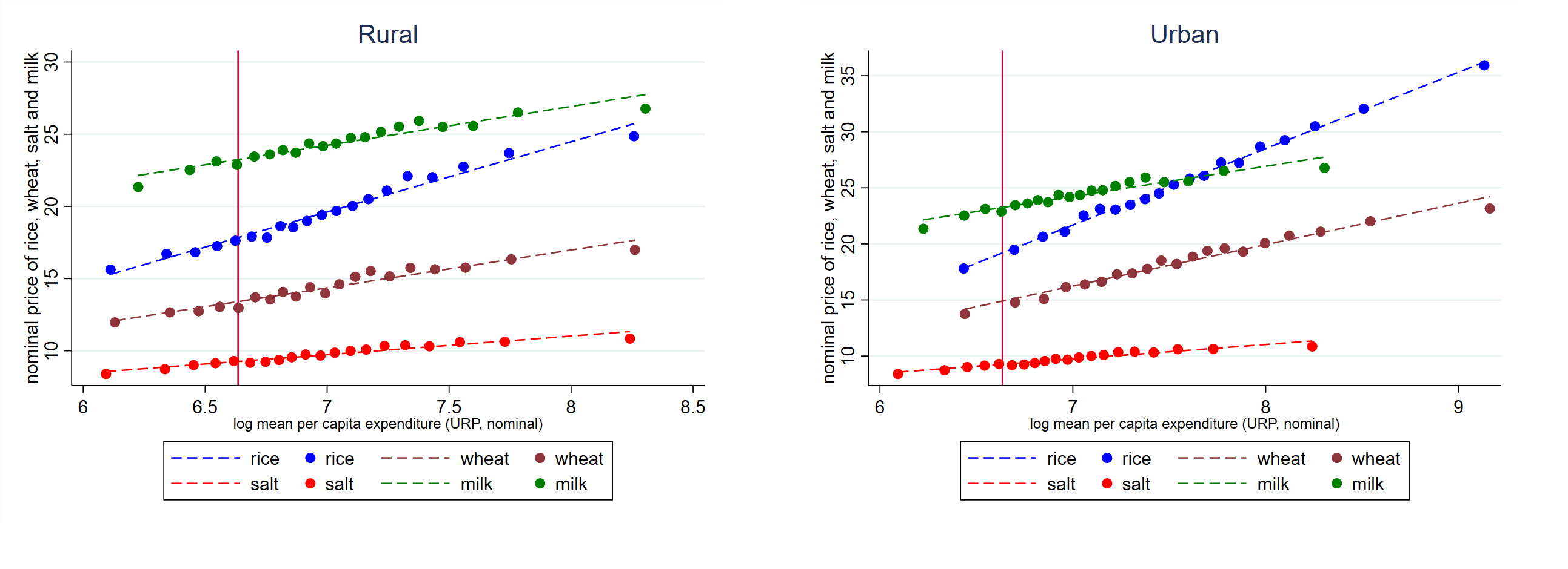
Notes: Unit prices are calculated as the ratio of household expenditure on items and quantities consumed in the 2011 round of CES. The unit price for rice and wheat depicted in the figure does not include household’s cereal consumption from the public distribution system. The scatter plots in the figure are averages calculated at 20 bin intervals while the fitted line is based on observed data; the figure is constructed using Stata’s binscatter function.
Incorporating food subsidies into the poverty calculation makes sense, but has to be done consistently
Another innovation adopted by BBV is that they value household expenditures on subsidized rice and wheat at market prices (rather than at the subsidized prices households purchased the rice and wheat for). This is by no means an unreasonable choice. It should be noted however, that this approach implies abstracting from quality differences between goods. To illustrate this, we regress the unit price of four choices of goods (rice, wheat, milk, and salt) against log household expenditure from the 2011 consumption expenditure survey of the NSS, see Figure 3. All expenditures concern market goods (i.e., purchase of subsidized rice and wheat are excluded). The slopes of the fitted lines arguably capture differences in both quality and location. Salt is included as a control as it represents the most homogenous good among the four with little to no variation in quality, such that the slope coefficient captures variation in location, not quality. Subtracting this slope for salt from the slopes observed for rice, wheat, and milk indicates that a notable degree of the variation in prices can be attributed to quality-differences, richer households on average purchase higher quality versions of the same good at higher prices. Deaton (1988) puts forward an approach to account for these quality differences.
Abstracting from quality differences for the purpose of poverty measurement is certainly a defensible choice. This choice has several important implications, however, that warrant further study. First, virtually every consumption good can be purchased at different quality levels and consequently exhibit variation in unit prices. Hence a consistent application of this approach would require one to apply the price adjustments across a wider set of goods (not just subsidized rice and wheat). Second, what price should one value the expenditures at? The average market price assumed by BBV is generally significantly higher than the average price households below or around the poverty line purchase the goods for in rural areas (see Figure 4). In urban areas, the assumed uniform prices are notably closer to (or just below) the nominal unit price paid by poor households. Third, the same price that is used to adjust household expenditure values should ideally also be used to adjust the value of the national poverty line. For example, the amount of rice included in the basic needs basket that underlies the poverty line should be evaluated at the same price. Using subsidized prices to value the poverty line but higher market prices to value household expenditures (as BBV currently does) will lead to an under-estimation of poverty. It should be noted that BBV adopt the international poverty line of $1.9 a day and hence do not have to evaluate the price of the basic needs consumption basket for India. By the same token, however, the international poverty line is derived from cross-country data on poverty lines that reflect the cost of acquiring the basic needs basket. Conceptually, this means that if one were to change the prices used to evaluate household expenditures, one would have to use the same prices to evaluate the cost of the basic needs basket to verify whether households can afford the basic needs consumption basket.
Figure 4: Selection of a uniform market price can impact estimates of poverty due to quality differentials
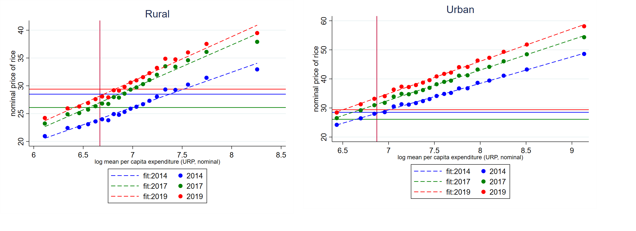
Figure Notes: Unit prices for 2014, 2017 and 2019 are calculated using the observed unit price of rice in CES 2011 round and the food price inflation reported in the CPI state (rural and urban) series – the BBV’s preferred choice of deflator series. The horizontal lines in different colors represent the price at which BBV value PDS consumption of rice. The vertical red line is the $1.90 poverty line – poor households are on the left of this line. The figure shows that in rural areas, the unit price of rice implied by state level CPI food indices is lower than the price rice assumed by BBV across years. This discrepancy will overestimate poverty reduction in rural areas but underestimate poverty reduction in urban. Since discrepancies are markedly larger in rural samples and rural population is about 67 percent of the overall population, the national poverty estimates at BBV’s assumed price levels likely overestimate average consumption and underestimate national poverty headcounts. As in Figure 3, the scatter plots indicate mean values across 20 bins using Stata’s binscatter function.
Note: BBV suggest that the targeting efficiency of India’s PDS program improved from 54 percent to 86 percent from 2014-15 onwards, citing Bhattacharya and Sinha Roy (2021). As a point of clarification, Bhattacharya and Sinha Roy (2021) finds that a high share of people across the welfare distribution were able to receive government transfers (while taking stock of the PDS transfers during the emergency covid period). For instance, 93.1 percent of poor eligible households received these transfer benefits in addition to 81 percent of eligible non-poor households. From these estimates alone, one cannot infer with what efficiency PDS transfers are allocated across households with different expenditures – and hence are not able to provide support for the assumed targeting efficiency estimate of 86 percent in BBV.
Acknowledgement: The authors are grateful to Andrew Dabalen, Christoph Lakner, Daniel Mahler, Berk Ozler, Carolina Sanchez Paramo for providing helpful comments and suggestions.
Disclaimer
CGD blog posts reflect the views of the authors, drawing on prior research and experience in their areas of expertise. CGD is a nonpartisan, independent organization and does not take institutional positions.